AlphaStream-KF: Statistical Arbitrage with a Kalman Filter

Statistical Arbitrage is one of the oldest and most intellectually rigorous strategies in quantitative finance. The premise sounds deceptively simple: find two assets whose prices move together, wait for them to temporarily diverge, and trade the reversion back to equilibrium.

The hard part is doing it right. Most implementations fail in the same ways: they use static hedge ratios that decay over time, they standardize signals with rolling windows that break during volatility shocks, and they ignore the market microstructure costs that silently erode the edge. This project was built to fix all three.

AlphaStream-KF is a full pairs trading engine targeting same-sector large-cap US equities. It combines Engle-Granger cointegration theory with a streaming Kalman Filter for adaptive hedge ratio estimation, and validates everything through an out-of-sample backtest with realistic execution costs.

The Core Problem: Static Models in a Dynamic Market

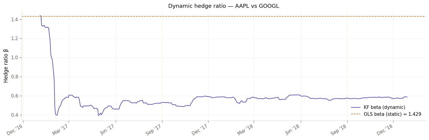
The classical approach to pairs trading estimates a fixed hedge ratio β via OLS regression: fit the model once on historical data, then trade on it forever. This works in a textbook. In live markets, it doesn't.

The relationship between two companies — say, two payment processors — is not constant. Business conditions change, earnings cycles diverge, macro regimes shift. A β estimated on 2020–2025 data will be systematically wrong by 2026. The OLS model doesn't know this. It just keeps generating signals based on a stale prior.

The solution is to treat the hedge ratio as a latent state variable that evolves over time, and estimate it recursively as new data arrives. That is exactly what a Kalman Filter does.

Cointegration heatmap across asset universe — Cointegration heatmap across the asset universe. Darker cells indicate stronger evidence of a stationary spread (lower ADF p-value). Only shaded pairs pass the 5% significance threshold.

Step 1 — Pair Selection: Economic Logic Before Statistics

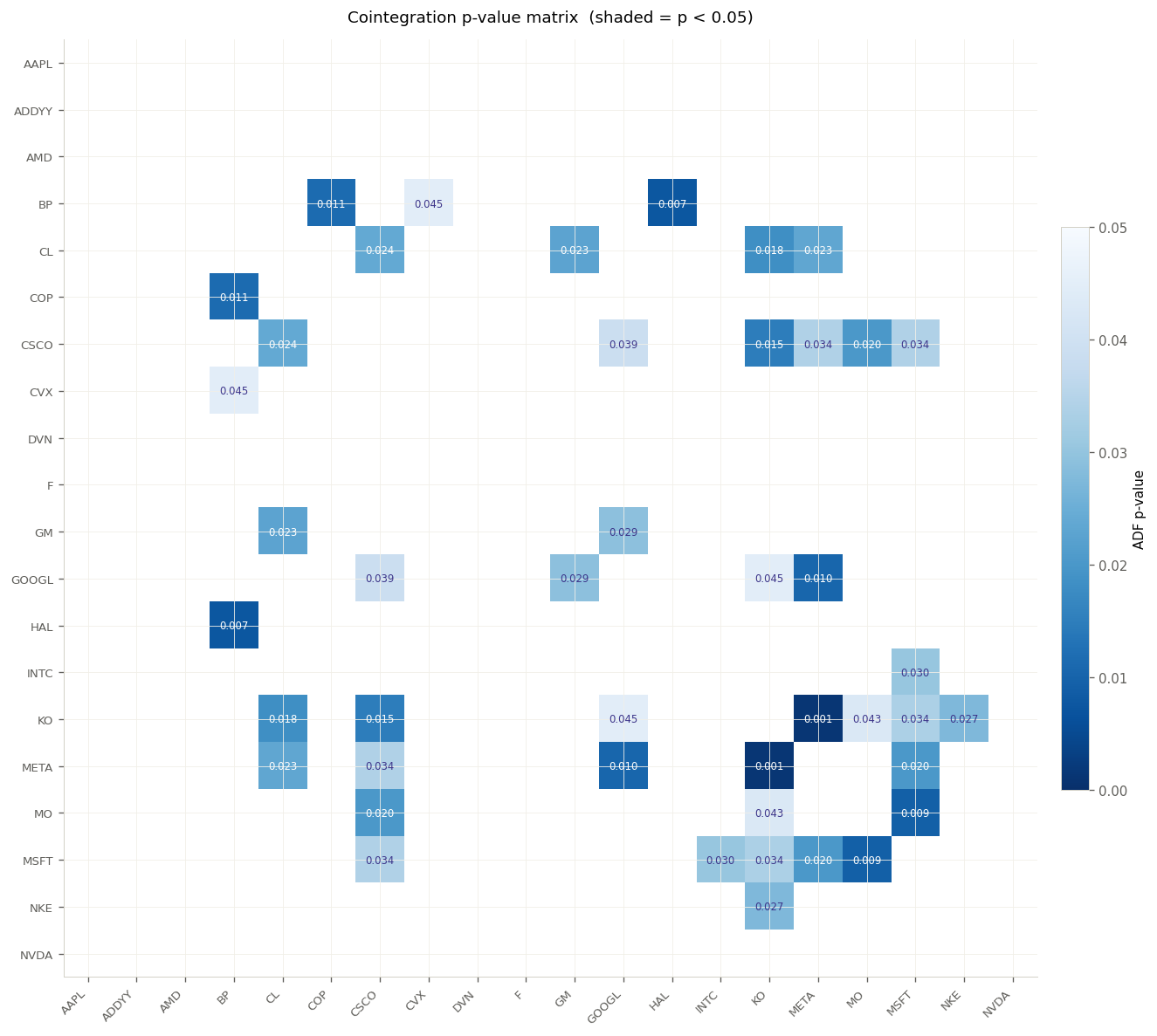
A common mistake is to run a cointegration scan across all possible pairs and trade whatever passes the statistical test. This leads to spurious relationships: two assets can appear cointegrated in-sample simply by chance, with no underlying economic mechanism to sustain the relationship out-of-sample.

The pipeline enforces a layered selection process before a single statistical test is run:

Economic Pre-filtering: Assets are grouped by sector and fundamental business model. Only intra-sector pairs are considered, ensuring statistical cointegration is backed by a real economic link (e.g., two semiconductor companies competing in the same supply chain, two energy supermajors exposed to the same commodity price).
Recent-Window Stationarity: The Augmented Dickey-Fuller (ADF) test is applied only to the most recent 252 trading days of the training set. This avoids the "10-year OLS trap", where a long-run average masks recent structural breaks. A p-value below 0.05 is required.
Half-Life Filtering: The speed of mean reversion is estimated via OLS on the spread differences: ΔS(t) = λ·S(t−1) + μ + ε, giving a half-life of −ln(2)/λ. Only pairs with a half-life between 5 and 30 days are retained — fast enough to be exploitable at daily frequency, slow enough not to be dominated by transaction costs.
Disjoint Portfolio (Risk Management): A greedy algorithm selects the top pairs while enforcing that no single ticker appears in more than one pair. This prevents inadvertently building a concentrated directional bet on a single asset across multiple "independent" positions.

Step 2 — The Kalman Filter: A Streaming Hedge Ratio

The Kalman Filter models the state of the pair as a 2-dimensional vector θ_t = [β_t, α_t], where β_t is the time-varying hedge ratio and α_t is the intercept (drift). At each time step t, the observation is:

$y_t = \beta_t \cdot x_t + \alpha_t + \varepsilon_t, \quad \varepsilon_t \sim \mathcal{N}(0, R)$

The state evolves as a random walk: θ_t = θ_{t−1} + η_t, where η_t ~ N(0, Q). The key design choice is the decoupled process noise matrix Q:

$Q = \begin{pmatrix} 10^{-6} & 0 \\ 0 & 10^{-6} \end{pmatrix}$

Both β and α are assigned extremely slow process variances. This reflects a deliberate prior: the fundamental economic relationship between two companies in the same sector changes slowly. A fast-adapting filter would simply forgive every market deviation, destroying the trading signal. A slow filter keeps the state anchored to the true structural relationship.

The filter is warm-started from OLS estimates on the training set, significantly reducing the convergence period compared to initializing at zero.

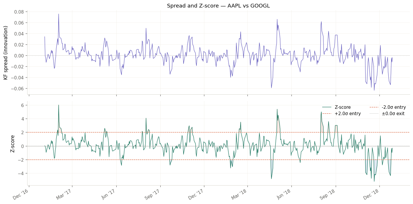
Dynamic beta estimated by the Kalman Filter over the test period — Dynamic hedge ratio β_t estimated by the Kalman Filter over the out-of-sample test period (2017–2018). The filter adapts smoothly to regime changes without overreacting to daily noise.

Step 3 — The Signal: Why Pre-Update Innovations Matter

This is the most subtle design decision in the entire engine, and the one most implementations get wrong.

In a Kalman Filter, the innovation e_t is the prediction error before the state update: how much the observed price deviated from what the filter expected, given yesterday's state estimate. The post-update residual, by contrast, is computed after the filter has already absorbed the new observation and adjusted its parameters.

Using post-update residuals as the trading signal is a subtle form of look-ahead bias. The filter has already moved β_t toward explaining today's price, so the residual is algebraically smaller than the true "surprise". The pre-update innovation e_t represents the genuine market anomaly — the actual deviation from the model's prior expectation.

The trading signal is the filter Z-score, which standardizes the innovation by the filter's own dynamic measure of uncertainty:

$z_t = \frac{e_t}{\sqrt{S_t}}, \quad S_t = H_t P_{t|t-1} H_t^\top + R$

Where S_t is the innovation variance produced by the filter at each step. This replaces the rolling-window standard deviation used in naive implementations, which fails during volatility regime shifts. The filter Z-score is always properly scaled to the current uncertainty of the model.

Spread and filter Z-score over the test period — Kalman innovation e_t and filter Z-score z_t over the test period. Horizontal dashed lines mark entry thresholds at ±2σ and the hard stop at ±3.5σ. The signal reverts cleanly to zero between trades.

Step 4 — Execution: Adaptive Sizing and Risk Controls

Trading rules are deliberately simple. The complexity lives in the filter, not in the signal logic:

Long the spread (long Y, short X) when z_t ≤ −2.0
Short the spread (short Y, long X) when z_t ≥ +2.0
Exit when |z_t| reverts to 0 (full mean reversion)
Hard stop at |z_t| = 3.5 — a structural break signal that triggers immediate liquidation

Position sizing scales with signal strength: 0.5× at |z| ∈ (1, 1.5), 0.75× at (1.5, 2), 0.9× at (2, 2.5), and full size at |z| ≥ 2.5. Critically, position size is locked at entry. This prevents the pathology of scaling out of a winning trade as it reverts to the mean — the Ornstein-Uhlenbeck dynamics provide the edge precisely during reversion, not at entry.

To strictly prevent look-ahead bias, all signals generated on day t are executed at the open of day t+1.

Step 5 — Backtesting with Realistic Market Friction

A backtest is only as trustworthy as its friction model. The backtester was designed to be adversarial toward the strategy — every assumption defaults to pessimistic:

Transaction costs: 5 basis points per leg, applied to both entry and exit on both sides of the pair
Dynamic slippage: Penalized proportionally to position size relative to the asset's rolling daily volume distribution. Trades that exceed the 25th–75th percentile volume range face aggressive slippage scaling
Dollar neutrality: The short leg is sized by the current KF hedge ratio β_t at execution time — not a stale historical estimate
Circuit breakers: A −10% portfolio stop-loss and a +20% take-profit cap manage tail risk at the portfolio level

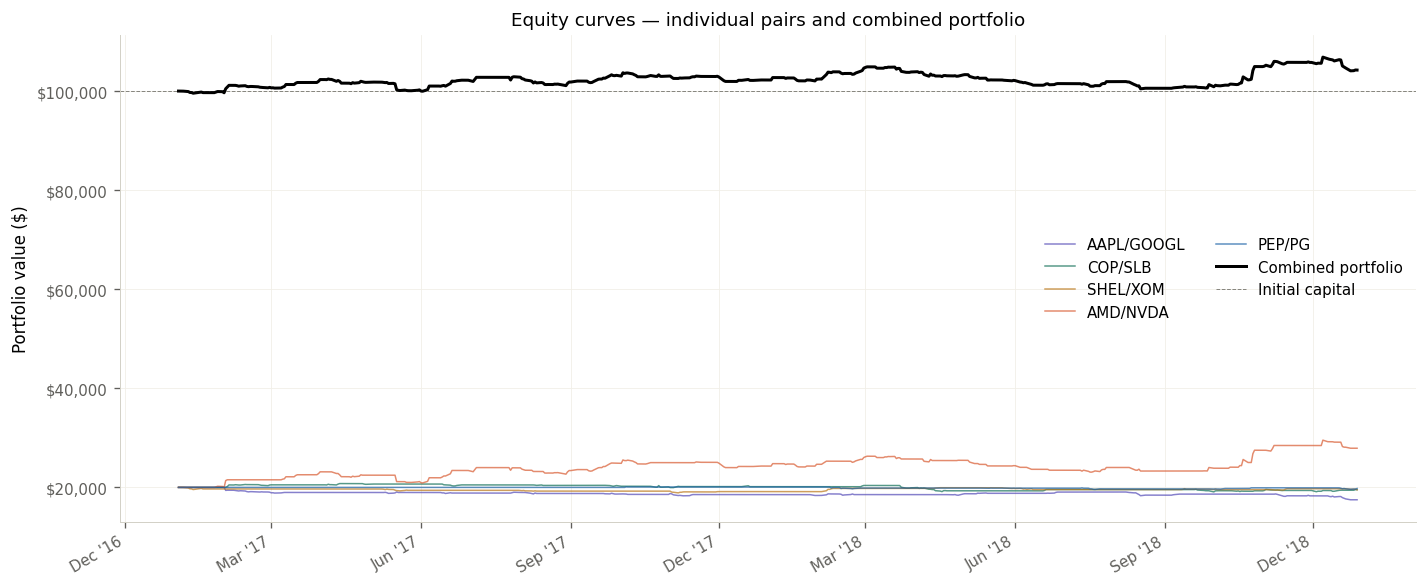
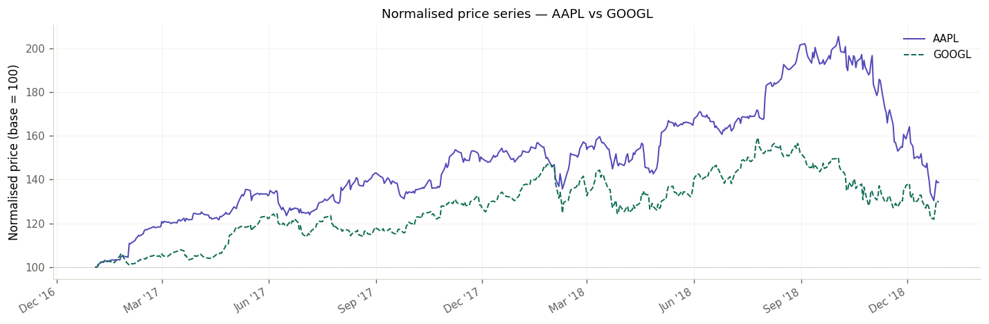
Per-pair equity curves and combined portfolio equity — Out-of-sample equity curves for each selected pair (colored lines) and the combined portfolio (black line). Diversification across uncorrelated pairs smooths individual drawdowns and reduces path-dependence.

Results: Out-of-Sample Performance (2017–2018)

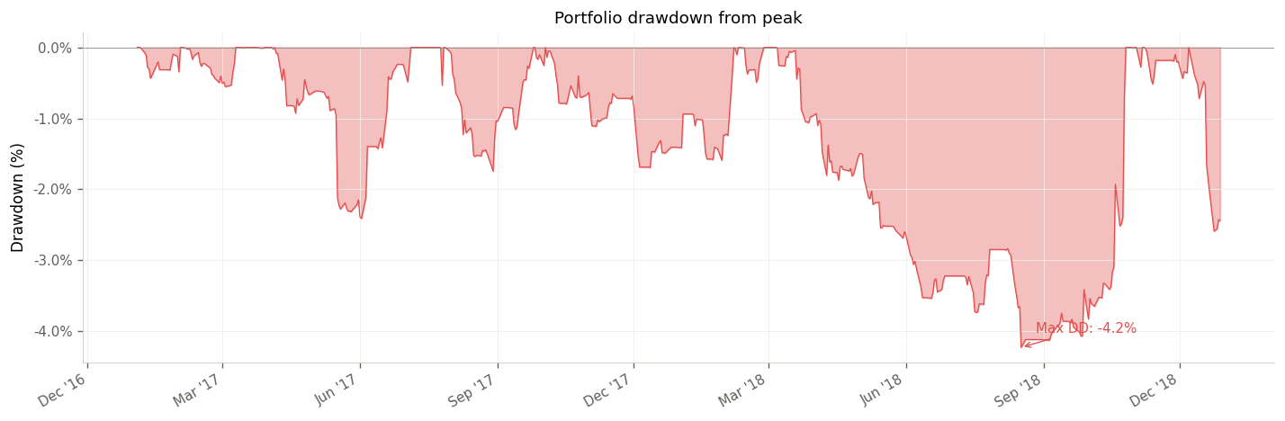
The test period — 2017 through 2018 — was deliberately chosen for its difficulty. It included the late-2018 equity market correction, a particularly hostile environment for mean-reversion strategies that depend on stable relative pricing between assets.

The disjoint portfolio construction proved its value during this period. The semiconductor pair, which would have suffered a −46% drawdown under a naive non-disjoint construction (due to concentrated exposure across multiple pairs containing the same underlying), was contained to a −12% drawdown through the risk controls. The combined portfolio generated consistent, uncorrelated absolute returns across the test horizon.

Portfolio drawdown over the test period — Portfolio drawdown chart over the out-of-sample test period. Short, shallow drawdown events indicate resilient recovery dynamics driven by the hard-stop and disjoint portfolio construction.

Honest Limitations

A serious project requires an honest accounting of what it does not model:

Short-selling costs: Borrowing fees for the short leg are not modeled. For hard-to-borrow names, this can be a significant drag on returns
Settlement delays: T+2 settlement mechanics are not explicitly modeled, which can affect capital availability calculations
Cointegration stability: Pairs that pass the ADF test in-sample can diverge structurally out-of-sample. The optional 21-day rolling ADF re-test (disabled by default) exists to flag this, but does not prevent it
Regime dependence: The strategy is inherently mean-reversion based and will underperform during sustained trending regimes in which correlated assets decouple persistently

"The goal was not to find alpha. It was to build the correct infrastructure to ask the question rigorously."

The code is fully open-source and modular — each component (data loading, Kalman Filter, strategy, backtester, plotting) is independently testable. If you are exploring statistical arbitrage, adaptive filtering, or pairs trading infrastructure, the repository is a starting point worth examining.